 Log In
Search




 Open Access
 yanrongguo@usst.edu.cn
Rongguo Yan, School of Health Science and Engineering, University of Shanghai for Science and Technology, No. 334, Jungong Road, Shanghai 200093, China. E-mail: yanrongguo@usst.edu.cn.
Received October 25, 2025; Accepted December 4, 2025; Published March 24, 2026
Open Accessyanrongguo@usst.edu.cnRongguo Yan, School of Health Science and Engineering, University of Shanghai for Science and Technology, No. 334, Jungong Road, Shanghai 200093, China. E-mail: yanrongguo@usst.edu.cn.
Received October 25, 2025; Accepted December 4, 2025; Published March 24, 2026
The 2024 China Cardiovascular Health and Disease Report pointed out that from 1990 to 2019, the incidence of cardiovascular disease (CVD) in China increased by 132.82% over that 30-year period [1]. CVDs are characterized by acute onset and high severity, which usually quickly lead to life-threatening events. Therefore, the early prevention and accurate diagnosis of CVDs are of great clinical significance.
Acoustic auscultation is a generally accepted initial screening method among the currently available diagnostic methods, which is non-invasive, convenient and cost-effective. Its clinical significance stems from the association between organic heart disease and abnormal heart sounds. The analysis of acoustic signals has reference value in the early detection and risk stratification of CVDs. However, traditional auscultation has limitations. Its effectiveness relies heavily on the experience of clinicians and involves subjective interpretation of findings, which lacks objectivity and standardisation. Consequently, these limitations hinder the screening of the whole population and compromise both the consistency and accuracy of diagnosis.
With the continuous and rapid development of digital signal processing and artificial intelligence technology, computer-aided diagnosis systems provide a new way to mediate the limitations of traditional auscultation. Through digital processing of sound signals, the computer-aided diagnosis system can automatically identify the typical characteristics of the sample and use intelligent learning algorithms to further improve the standardisation and reliability of its voice processing. Subsequently, this can improve the accuracy in detecting abnormalities and the consistency of clinical diagnosis.
The general process of heart sound classification includes three stages: preprocessing, feature extraction, and classification model training. Preprocessing is mainly used for denoising and segmentation, while feature extraction and model design are key to achieving high classification performance. The current methods for classifying heart sounds can be roughly divided into three categories: traditional methods based on manual features, methods based on deep learning, and methods based on multi-feature fusion.
Early research relied heavily on manually designed features combined with traditional classifiers.
For example, Li et al. used wavelet transform and Twin Support Vector Machine to achieve heart sound recognition; Xu et al. integrated time-domain and frequency-domain features with random forest and AdaBoost to classify congenital heart disease in children; Taneja et al. used gammatonegram features combined with a support vector machine (SVM) to achieve heart sound classification [2-4]. Although these methods can achieve certain results, they are difficult to capture complex temporal patterns.
With the development of deep learning, researchers have begun to use neural networks to automatically extract high-level features. Rubin et al. combined mel-frequency cepstral coefficients (MFCCs) with convolutional neural networks (CNNs); Deng et al. proposed a Convolutional Recurrent Network based on improved MFCC; Shahid et al. used spectrograms combined with CNN and SVM for heart sound classification; Xiao et al. and Oh et al. directly used the original heart sound signal as input and implemented end-to-end classification using an attention mechanism or WaveNet [5-9]. Li et al. developed the Multi-scale DenseNet and Multi-head Attention Recurrent Neural Network (MDN-MARNN) model, which uses a multi-scale DenseNet structure and a multi-head self-focus RNN, which is an end-to-end classification method based on error label data with a certain degree of interpretability [10]. Patwa et al. proposed a composite 1D-CNN and wavelet scattering transformation (WST) model, which provides robustness under small sample testing and class imbalance [11]. Cheng et al. proposed the CNN-Transformer End-to-end Neural Network (CTENN) model, which utilizes CNN to extract local features and Transformer to capture global dependencies, achieving end-to-end heart sound classification and performing well on the PhysioNet dataset [12]. Compared to traditional methods, these models significantly improve feature learning ability and classification performance.
In recent years, multi-feature fusion has emerged as a new research focus. This type of method enhances the ability to characterize heart sound signals by integrating features of different types or levels. Abbas et al. fused spectrograms with MFCC to enhance robustness; Lee et al. combined wavelet transform and CNN to achieve multi-scale feature extraction; Li et al. proposed the CAFusionNet model, which significantly improves classification accuracy through multi-layer feature fusion and a channel attention mechanism [13-15]. Overall, the introduction of multi-feature fusion and attention mechanisms provides new research directions and performance breakthroughs for intelligent classification of heart sounds. Khan et al. proposed a heart sound spectrogram classification method based on residual learning and multi-model feature fusion [16]. MobileNet and DenseNet201 were used to extract features and residual fusion was used to enhance the model expression ability. The method achieved excellent heart rhythm anomaly detection performance on both PhysioNet 2016 and BreakHis datasets, and was combined with Gradient-weighted Class Activation Mapping to provide model interpretability.
In two-dimensional acoustic representation, MFCC features are still one of the most common features due to their perceptually motivated spectral representation. Nevertheless, traditional MFCCs only represent, i.e., characterise, the spectral envelope of a selected frame, and thus do not capture the temporal dynamics of heart sounds. In this study, dynamic MFCC features are derived to capture the temporal dynamics. Furthermore, these dynamic MFCCs are visualised to generate dynamic MFCC feature map. These dynamic MFCC feature maps are then used to construct and integrate two feature extraction models, the outputs of which are combined and classified using an SVM classifier. Consequently, the proposed approach improves the robustness and accuracy of heart sound classification by effectively combining temporal dynamic and spectral representations.
2.1 Static MFCC
MFCC is one of the most common acoustic characteristics in biomedical signal and speech processing. It represents the perceptual characteristics of the human auditory system, and its frequency response is nonlinear, because people are more sensitive to low frequencies than to high frequencies. MFCC uses the Mel scale to model this perceptual nonlinearity, making it an appropriate representation of the spectral envelope of sound signals [17, 18]. The workflow of MFCC feature extraction is illustrated in Figure 1.

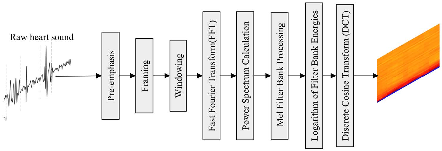
The pre-emphasis in the heart sound classification is to enhance the high-frequency component and reduce the low-frequency energy at the same time. This improves the detection of subtle changes and pathophysiological information that are usually embedded in high-frequency bands. Pre-emphasis is defined as the following equation:

Where x(n) is the original signal, y(n) is the pre-emphasis output, and the pre-emphasis coefficient α is usually between 0.9 and 1.0.
Heart sound is a quasi-stationary signal, which allows the original heart sound to be divided into short, overlapping time frames to enable spectral decomposition of each frame. In order to maintain continuity and reduce spectral leakage, each time frame is multiplied by a window function. In heart sound processing, the Hamming window and Hann window are usually used as window functions. Although their functions are similar, the Hamming window has a wider main lobe and better stopband roll-off, which allows for flexible suppression of side lobe influence. In contrast, the Hann window usually has better resolution and narrower side lobes (which also have lower amplitude) [19]. The Hamming window can be mathematically represented as:

When segmenting the heart sound signal, parameters such as segment duration (t), sampling frequency (fs), frame length (Fl), and frame shift (Fm) must be considered, as they determine the total number of frames M, given by:

Since heart sound signals exhibit less distinct time-domain features, it is necessary to analyze their spectral content. A Fast Fourier Transform is applied to each windowed frame to convert the signal from the time domain to the frequency domain:

The power spectrum provides a quantitative measure of energy distribution across frequencies, reflecting cardiac activity intensity at each frequency component:

The Mel filter bank is designed to approximate the human auditory perception of frequency. The conversion from frequency f(Hz) to the Mel scale is expressed as:

The inverse conversion from Mel scale to frequency is given by:

Each Mel filter has a triangular response, with a maximum at the center frequency and overlapping ranges between adjacent filters to ensure smooth spectral coverage. The transfer function of the mth Mel filter is defined as:
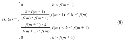
Where f(m) denotes the center frequency of the mth filter, f(m-1) and f(m+1) represent the lower and upper bounds, respectively. These frequencies are computed as:

Where S is the number of sampling points, fs is the sampling frequency, and fl and fh are the lowest and highest filter frequencies, respectively.
Because human auditory perception is logarithmic in amplitude, the Mel filter output is transformed logarithmically to simulate perceived loudness. The spectral energy at the output of the mth Mel filter is calculated as:

Finally, applying a Discrete Cosine Transform (DCT) to the logarithmic Mel energies produces the MFCC coefficients:

DCT organises the signal energy in a set of low-order coefficients, which are appropriately related to the characteristics and significantly reduce the dimension of the data, which makes the subsequent classification tasks more robust and efficient.
2.2 Dynamic MFCC
Dynamic MFCCs enhance the traditional static MFCCs representation by incorporating temporal change information of the signal. Static MFCC coefficients are essentially equivalent to instantaneous acoustic characteristics, as they represent the spectral envelope of the signal within a single frame. However, they do not capture the temporal evolution of the signal's characteristics. In contrast, physiological signals such as voice and heart sound are characterised by strong time continuity, and the transition between states contains important diagnostic or classification information.
To explain this limitation, we only need to use first-order and second-order derivatives, Delta characteristics and Delta-Delta characteristics respectively. These quantify the speed and acceleration of spectral features and enhance the ability of the model to capture dynamic time characteristics.
The first-order difference (Delta feature) represents the rate of change of an MFCC coefficient over time, approximating its first-time derivative and indicating the envelope of transition between frames. Mathematically, this is expressed as:

Here, ct(n) is the nth coefficient of MFCC at frame t, Δct(n) is the first-order difference of ct(n) (or Delta coefficient), and K is the regression window size (which defines the temporal context by including adjacent frames). K is the time offset weight, which determines the impact of previous and current time frames.
The second-order difference (Delta-Delta characteristic) is the first-order rate of change of the Delta coefficient, which captures the acceleration of MFCC evolution and thus represents the second-order rate of change of MFCCs. The calculation of Delta features applies a differentiation operation:

Similarly, this encapsulates the second-order temporal dependence of the rate of change of spectral characteristics—a desirable feature to describe transient or periodic characteristics in heart sound signals.
2.3 Deep residual network (ResNet) 18
The ResNet was first introduced by He et al. in 2015, representing a major milestone in the design of deep neural networks [20]. A major innovation of ResNet is the use of residual connections, which mitigate the vanishing gradient problem and alleviate network degradation in deep networks during training. Thus, it enables the design of deeper and more stable architectures. Since its design, ResNet has achieved great success in many fields, including image classification, speech recognition and medical signal analysis. The basic/residual block is shown in Figure 2.
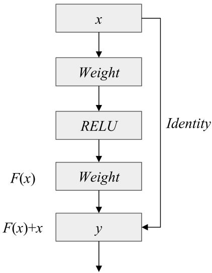
As shown in Figure 2, the residual block is formed by two paths: the residual mapping path composed of multiple layers (convolution, batch normalization, rectified linear unit, etc.), represented by F(x), and the identity mapping path, in which the input x is directly passed to the output through the so-called skip connection. The output calculation of the residual block h(x) is as follows:

Here, F(x) represents the nonlinear transformation of input x. The original input x is directly added to F(x) via the skip connection, which allows direct feature propagation.
ResNet18 is one of the most prominent and simplest models in the ResNet family, comprising 18 layers. The architecture aims to trade some feature extraction capabilities to keep parameter counting and computing complexity relatively low, allowing it to be used for small-scale data sets (and/or embedded devices). The overall structure of ResNet18 is shown in Figure 3.
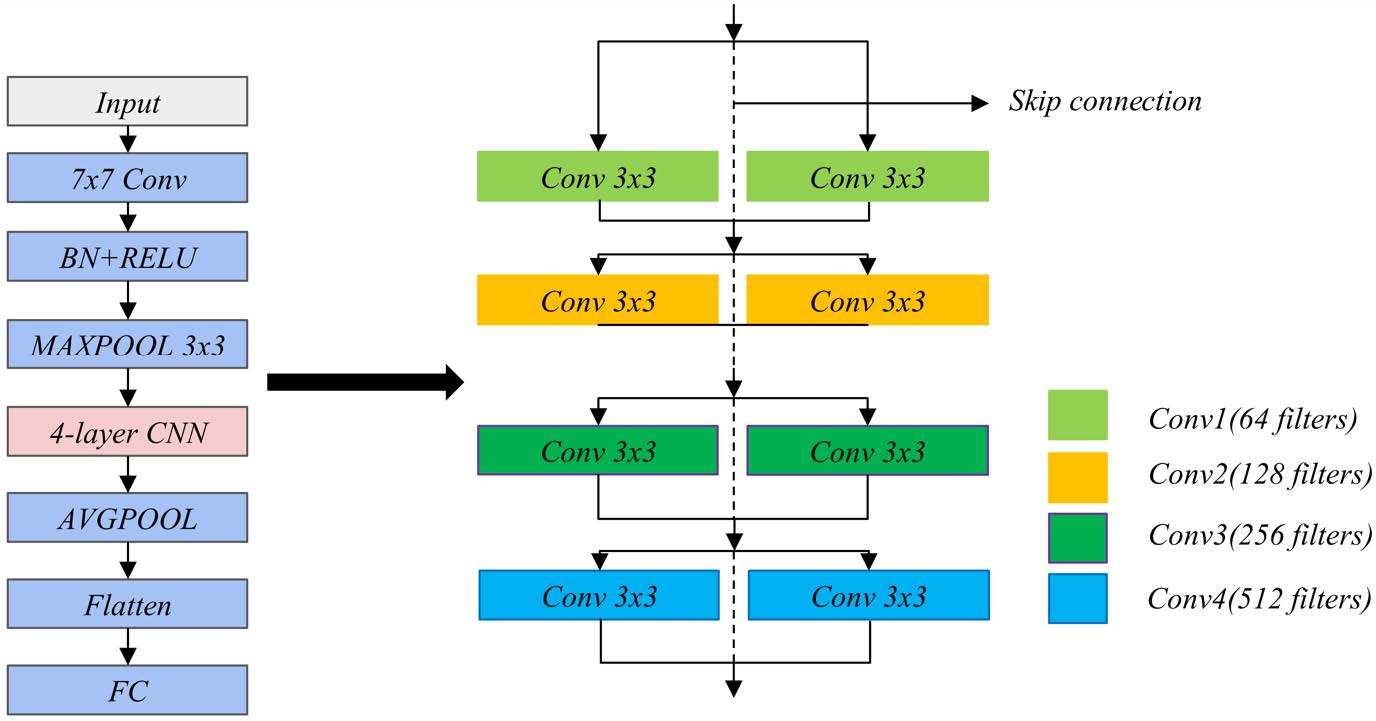
Figure 3. ResNet18 architecture. Conv, convolution; BN, batch normalization; RELU, rectified linear unit; MAXPOOL, max pooling; AVGPOOL, average pooling; FC, fully connected (layer).
2.4 Attention mechanisms
The attention mechanism enables the deep learning model to focus on useful features while suppressing unrelated features and improving the performance of the model’s representation learning and classification [21, 22]. Three types of attention modules are used in this work: frequency attention, Multi-Head Attention (MHA) and Coordinate Attention (CA).
2.4.1 Frequency attention mechanism
The frequency attention mechanism is designed for time–frequency representations such as MFCCs. It focuses on the frequency dimension to highlight discriminative spectral components.
Given an input feature map X∈RC×F×T, temporal information is aggregated using global average pooling:

Then, two 1×1 convolutional layers with nonlinear activations generate frequency-wise attention weights:

Finally, the input features are reweighted by the attention map:

This mechanism adaptively enhances informative frequency bands while suppressing redundant information.
2.4.2 MHA mechanism
The MHA mechanism, introduced in the Transformer architecture, captures dependencies across multiple representational subspaces [23].
For input sequence X, the query, key, and value matrices are computed as:

The attention output is then obtained as:

Multiple attention heads are computed in parallel and concatenated:

This structure enables the model to learn richer contextual relationships and improve generalization.
2.4.3 CA mechanism
The CA mechanism is a lightweight module that encodes both channel relationships and precise positional information by decomposing spatial attention into two independent directions—horizontal and vertical [24, 25].
Given an input feature map X∈RC×H×W, CA first applies global average pooling along the height and width dimensions:
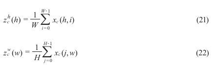
The pooled features are concatenated and passed through a shared 1×1 convolution and rectified linear unit activation for feature transformation:

The transformed feature is then split into two tensors, corresponding to the horizontal and vertical directions.

Two independent 1×1 convolutions with sigmoid activations generate directional attention weights:

Finally, the input feature map is reweighted by the corresponding attention weights to produce the refined output:

Using this separable coding method, CA captures long-range spatial dependencies while maintaining accurate location information and feature representation with lower computational complexity.
2.5 SVM
SVM is a supervised learning type model based on statistical learning theory. It develops an optimal hyperplane to maximise the separation between classes by establishing a large margin represented by a set of examples in a high-dimensional feature space. SVM learns a hyperplane, which provides powerful generalisation and classification performance based on structural risk minimisation.
Given a training set:

SVM seeks the optimal parameters w and b by solving the following optimization problem:

Using the Lagrange multiplier method, the dual form is expressed as:

Where ai are the Lagrange multipliers, and C is the penalty factor.
The final decision function is given by:

This formula allows SVM to use any number of kernel functions, such as linear, polynomial and radial basis function kernels, to effectively handle both linear and nonlinear classification tasks.
Multi-Branch Fusion MFCC (MB-FusionMFCC) model
In this work, we propose a MB-FusionMFCC to utilise the temporal dynamics of heart sound signals. Compared with previous methods that directly concatenate and classify MFCCs along with their first- and second-order derivatives, we treat the three feature types—static MFCCs, Delta coefficients, and Delta-Delta coefficients—as independent input branches, enabling each branch to learn representations specific to its characteristics. The model introduces a cross-branch attention model to improve the interaction and integration of feature types. The overall architecture is presented in Figure 4, and the detailed structure of each branch is shown in Figure 5.
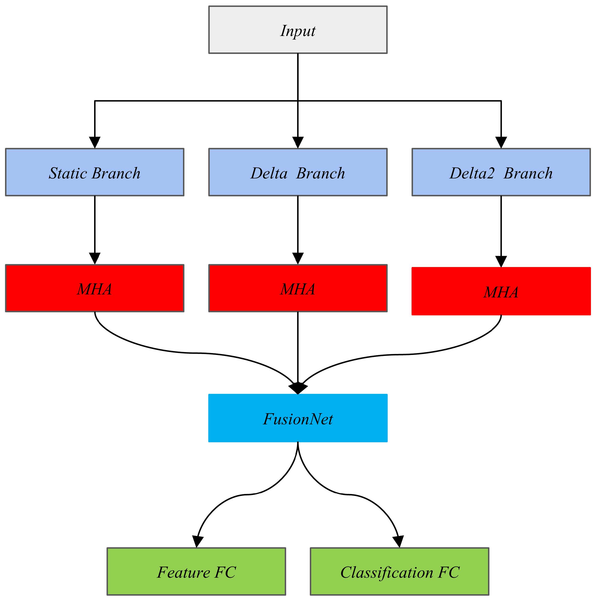
Figure 4. MB-FusionMFCC structure. Each branch shares the same architecture, which consists of three key modules: (1) a convolutional feature extraction module, (2) a frequency attention module, and (3) a global feature mapping module. MHA, Multi-Head Attention; FC, fully connected (layer); MB-FusionMFCC, multi-branch fusion mel-frequency cepstral coefficient.
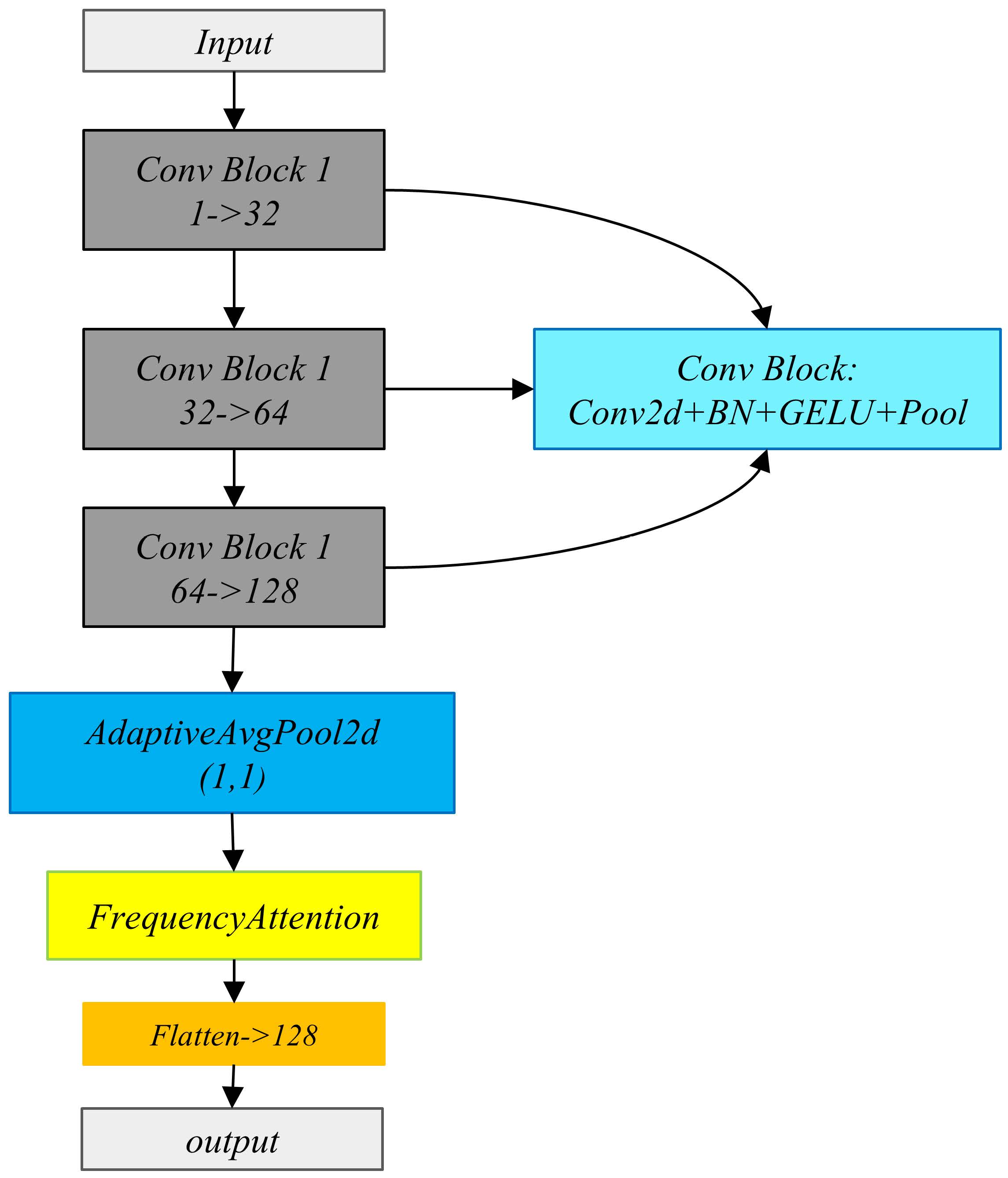
Figure 5. Branch structure. Conv, convolution (layer); BN, batch normalization; GELU, gaussian error linear unit; Pool, pooling (layer); AdaptiveAvgPool2d, adaptive average pooling 2D.
The convolutional feature extraction module is composed of a series of convolutional, batch normalisation, gaussian error linear unit, and pooling layers, enabling the model to learn time-frequency hierarchies.
The frequency attention module performs global pooling across time dimensions to learn the adaptive weighting of the frequency band, allowing the model to emphasize more discriminative frequency components for classification.
The global feature mapping module executes the global average pool and uses a fully connected projection to compress the two-dimensional feature map into a fixed-length vector to form a compact identification feature embedding.
The outputs of all branches are then integrated via a cross-branch attention module, which captures interactions among different feature representations by generating an attention-weighted fusion. Finally, the representation of cross-fusion is connected, then exited through the fusion layer, and then normalised through the weight mapping process.
The final result is to classify the final fusion feature vector into the heart sound category. It is also very reasonable to suspect that this advanced fusion representation may also exist in other tasks, such as diagnostic tasks or feature visualisation.
2.6 CA-ResNet18
This study uses CA-ResNet18, a CNN augmented with a CA fusion module, to extract the characteristics of classification tasks with dynamic MFCC feature images. The model is based on the structure of the standard ResNet18. By including the CA module, the model enhances the sensitivity to informative regions and the awareness of positional information within the spatial feature maps for classification.
Compared with the standard channel attention mechanism, the CA module pays global context attention to the height and width location information, while maintaining the location information of the spatial feature map. More importantly, the CA module decomposes spatial information through separate horizontal and vertical pooling on the 2D feature map, then globally encodes and recalibrates the features. This provides spatially-aware attention weights that enhance task-relevant regions.
In terms of architectural design, CA-ResNet18 uses the original definition of the ResNet18 residual block, but includes the CA module in the third (layer 3) and fourth (layer 4) stages of the model. Each residual unit is designed to first extract local features with convolution and batch normalization layers, and then use the CA module to provide joint channel attention and spatial attention for map features, so as to improve discrimination ability and robustness. Figure 6 shows the structural representation of the remaining units containing the CA module.
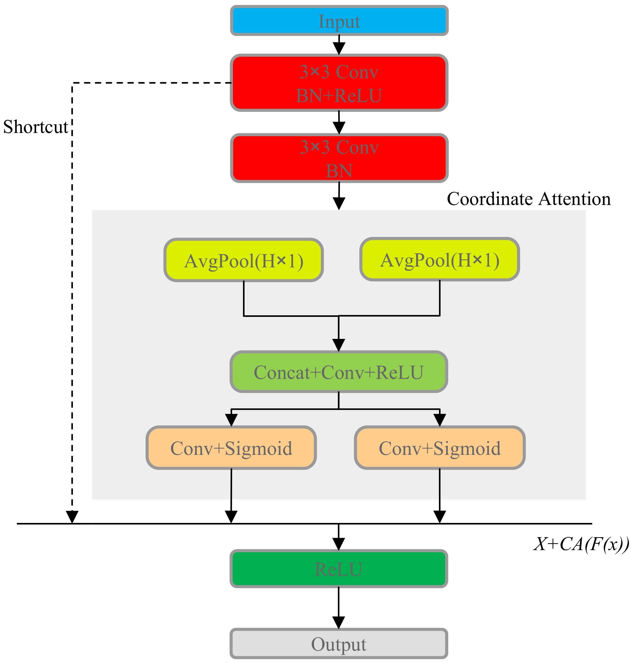
Figure 6. Residual unit structure after CA module embedding. CA, Coordinate Attention; Conv, convolution (layer); BN, batch normalization; ReLU, rectified linear unit; AvgPool, average pooling; Concat, concatenation (operation).
3.1 Experimental setup
The experimental simulation platform is configured using PyCharm Professional 2024.2.4, and the network is trained and evaluated on the PyTorch framework. The hardware includes NVIDIA RTX 4080 SUPER GPU, AMD Ryzen 9 9950X 16-core CPU, running Windows 11 and Python 3.9 as the programming language.
The model performance evaluation is carried out using five-fold cross-validation, which divides the dataset into five folds of equal size to maintain the same proportion of normal and abnormal heart sounds. In each iteration, one fold is regarded as a test set, and the remaining four folds are regarded as a training set to fully evaluate the generalisation ability of the model.
3.2 Evaluation metrics
The proposed method evaluation is carried out using the standard classification indicators of accuracy (Acc), sensitivity (Se), specificity (Sp), precision (Pre) and F1 score (F1). The definitions of these indicators are as follows:
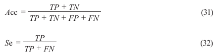
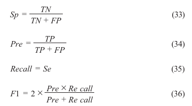
Here, TP, TN, FP and FN are used to indicate true positive, true negative, false positive and false negative respectively. These indicators together evaluate the accuracy of classification and the performance of the model in classifying abnormal heart sounds.
3.3 Dataset
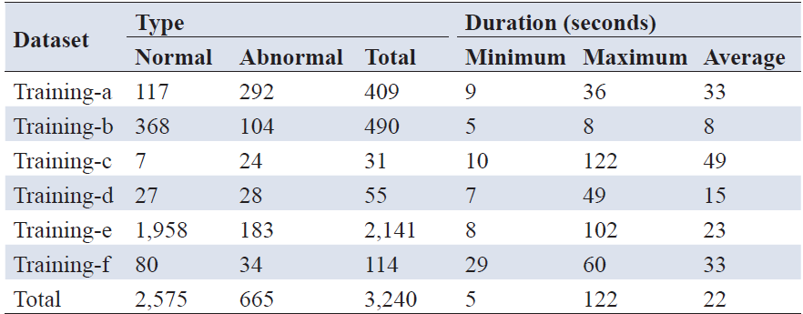
The experiment was conducted on the public dataset from the 2016 PhysioNet/CinC Challenge, which comprises six subsets with a total of 3,240 heart sound recordings. Of these, 2,575 recordings are considered normal heart sounds, and 665 are considered abnormal heart sounds [26]. The length of each heart recording ranges from 5 seconds to 122 seconds, and the sampling rate is 2 kHz. For each subset, the distribution of heart sound recordings is shown in Table 1.
3.4 Data preprocessing
Data preprocessing in this study consists of three main steps: filtering, segmentation, and normalization.
First of all, the data shows that the acquisition noise is mainly related to the stethoscope rubbing the subject’s skin at the beginning and end of recording. Therefore, the first second of each recording at both the beginning and the end has been deleted. The heart sound signals are segmented into three-second fragments, and any fragments shorter than three seconds are discarded. The signal is band-pass filtered using a 20-400 Hz fifth-order Butterworth filter to minimise high-frequency noise while maintaining the main frequency component of the heart sound signal.
Secondly, the dataset shows a strong imbalance, and the normal sample is much richer than the abnormal sample. Therefore, a targeted data balance strategy has been implemented. For normal samples, a fragment was obtained from each record, and for abnormal samples, four fragments were obtained to try to balance the representativeness of the minority. The datasets of training, verification and testing are divided at the patient level to avoid the overrepresentation of any individual sample and eliminate the overlap between patients.
Finally, all fragments of the heart sound are normalised in range to unify the numerical scale across samples to prevent gradient instability due to large amplitude denaturation, which helps to provide the convergence of the model and ultimately improve the classification performance.
3.5 MFCC static and dynamic feature extraction
Once the data is preprocessed, the MFCC characteristics are extracted. Each three-second segment is sampled at 2,000 Hz, then divided into overlapping frames of 256 samples with a frame shift of 64 samples, generating about 90 time frames.
Each frame is converted to the frequency domain by applying Fast Fourier Transform, and then the Mel filter bank is used to compute the logarithmic power spectrum. The resulting logarithmic power spectrum runs through DCT, and the 13-dimensional static MFCC coefficient is obtained.
From the static MFCCs, the first-order and second-order difference characteristics are calculated to characterise the time dynamics of spectral changes. These estimates are connected with static coefficients to produce a three-dimensional dynamic MFCC feature vector with 39 characteristics. In addition, all features have been normalised on a scale to ensure consistent statistical scaling across samples and produce a unified input format that can be visualised to develop training methods.
3.6 Extraction of static and dynamic MFCC feature images
After obtaining the 39-dimensional dynamic MFCC feature, all the feature vectors corresponding to the given time frame are connected in series according to the time order corresponding to x, and a two-dimensional matrix of size (39, 90) is generated, of which 39 corresponds to the frequency dimension and 90 is the time frame number, which acts as a heart sound signal. The two-dimensional time frequency is presented, and the time evolution of the spectral energy distribution is presented.
The matrix is linearly normalised to eliminate the amplitude changes of all samples in the pseudo-colour image. Then the normalised and numerically grounded components are quantitatively mapped to pixels in order to extract the two-dimensional demonstration of pseudo-colour and visually distinguish the characteristics. Compared with static MFCC images, dynamic MFCC images incorporate first- and second-order differential information into the original spectral structure, thereby capturing both instantaneous and transitional acoustic characteristics. This enriched representation provides deeper temporal context and a more discriminative feature space for deep neural network learning, the example of dynamic MFCC feature images is presented in Figure 7.
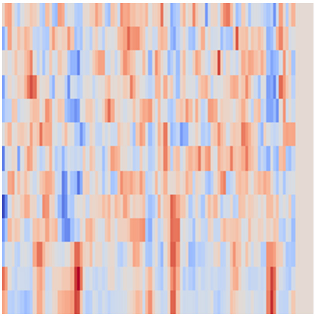
Figure 7. Examples of dynamic MFCC feature images. MFCC, mel-frequency cepstral coefficient.
4.1 Heart sound classification based on single features
In classification tasks based on MFCC and image features, CNNs and their derived architectures remain the most representative mainstream frameworks. To further evaluate the performance of the proposed models, Tables 2 and 3 present the classification results of the MB-FusionMFCC and CA-ResNet18 models compared with several typical CNN models and their improved variants.
Table 2. Performance comparison of different CNN models on dynamic MFCC features
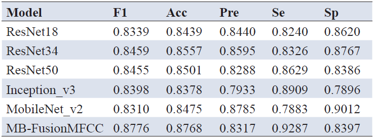
Note: Acc, accuracy; Pre, precision; Se, sensitivity; Sp, specificity; MB-FusionMFCC, multi-branch fusion mel-frequency cepstral coefficient; CNN, convolutional neural network; MFCC, mel-frequency cepstral coefficient.
Table 3. Performance comparison of different CNN models on dynamic MFCC image features
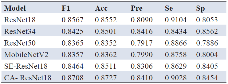
In the classification tasks using dynamic MFCC features and dynamic MFCC image features, the experimental results show that CNNs and their improved variants can effectively extract discriminative representations, though performance differences exist across architectures. For dynamic MFCC features, the MB-FusionMFCC model outperforms the traditional ResNet series, Inception_v3, and MobileNet_v2 in both F1-score and accuracy, indicating that its multi-branch fusion structure enhances the representation capability of MFCC features.
For dynamic MFCC image features, CA-ResNet18 achieves better performance than the original ResNet18 and other attention mechanisms (e.g., Squeeze-and-Excitation, Efficient Channel Attention), demonstrating that the CA mechanism helps capture both local and global dependencies in time–frequency representations.
Next, we introduce an SVM classifier on top of the existing models, where deep learning is used for feature extraction, and SVM serves as a lightweight classifier for final decision-making. The results are shown in Tables 4 and 5.
Table 4. Performance comparison of different CNN-SVM models on dynamic MFCC features
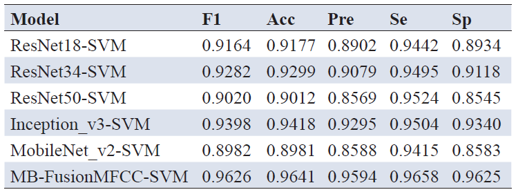
Note: Acc, accuracy; Pre, precision; Se, sensitivity; Sp, specificity; CNN, convolutional neural network; MFCC, mel-frequency cepstral coefficient; SVM, support vector machine; MB-FusionMFCC, multi-branch fusion mel-frequency cepstral coefficient.
Table 5. Performance comparison of different CNN-SVM models on dynamic MFCC image features
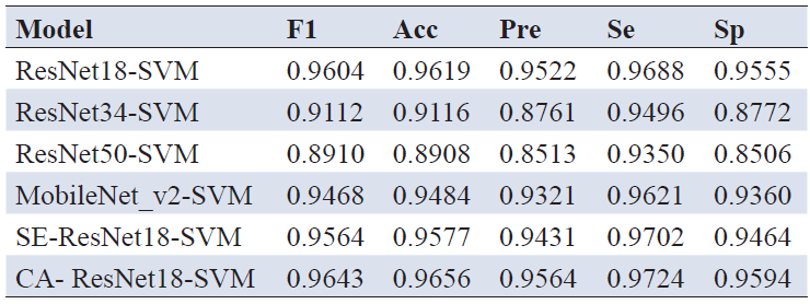
Note: Acc, accuracy; Pre, precision; Se, sensitivity; Sp, specificity; CNN, convolutional neural network; MFCC, mel-frequency cepstral coefficient; SVM, support vector machine; SE-ResNet18, ResNet18 with Squeeze-and-Excitation module; CA-ResNet18, ResNet18 with Coordinate Attention module.
4.2 Heart sound classification based on dynamic MFCC and dynamic MFCC image feature fusion
In the preceding sections, independent classification experiments were conducted using MB-FusionMFCC-SVM and CA-ResNet18-SVM for dynamic MFCC features and dynamic MFCC image features, respectively. Both models show high classification accuracy, which shows that they have strong feature representation and discrimination in both the time domain and the time-frequency domain.
Heart sound samples are used to extract advanced feature vectors through MB-FusionMFCC and CA-ResNet18 models. Each feature set is normalised before being connected together, resulting in a fusion feature representation. Fusion feature vectors are accessed by the SVM classifier for final classification.
Table 6 summarises the classification performance of the fusion feature model and the single feature model, and shows the benefits of multimodal feature fusion for heart sound classification.
Table 6. Classification performance comparison between fusion feature and single feature models

Note: Acc, accuracy; Pre, precision; Se, sensitivity; Sp, specificity; MFCC, mel-frequency cepstral coefficient; SVM, support vector machine; MB-Fusion MFCC-SVM, multi-branch fusion MFCC model with SVM classifier; CA-ResNet18-SVM, Coordinate Attention ResNet18 with SVM classifier; Fusion-SVM, fusion model with SVM classifier.
It can be seen from the survey results that when these features are input into Fusion-SVM, the combination of features extracted from the two models exceeds the single-modal use case. In order to check the validity of the proposed feature combination method, it was compared with the existing models, which represent the cross-section of the cardiac sound classification model in the current literature. Table 7 summarises the performance of the proposed model and the existing model trained on the common public data set (PhysioNet 2016 public dataset).
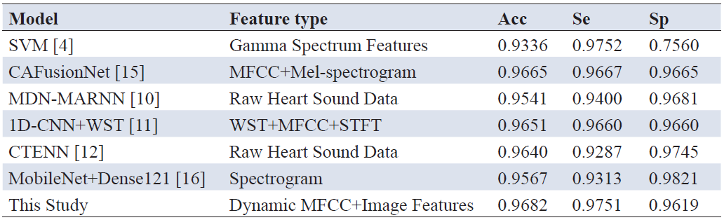
Note: Acc, accuracy; Se, sensitivity; Sp, specificity; SVM, support vector machine; MFCC, mel-frequency cepstral coefficient; CAFusionNet, Channel Attention fusion network; MDN-MARNN, Multi-scale DenseNet–Multi-head Attention Recurrent Neural Network; 1D-CNN, 1D-convolutional neural network; WST, wavelet scattering transform; CTENN, CNN-Transformer End-to-end Neural Network; STFT, short-time fourier transform.
As shown in Table 7, our cardiac sound classification method uses dynamic MFCC characteristics and dynamic MFCC images to show very high accuracy, sensitivity and specificity. The accuracy of the proposed method reaches 0.9682, which is comparable to other recent methods (for example, CAFusionNet, Acc=0.9665), demonstrating its competitiveness in modern heart sound classification. Reference 4 was among the first to introduce gamma spectral features using the SVM classifier, and achieves an accuracy of 0.9336. The contribution of reference 4 lies in the design of features. However, its low specificity (0.7560) may be due to class imbalance. The models in MDN-MARNN and CTENN takes fragments of the original heart sound, which allows them to extract time characteristics globally [10, 12]. However, potentially due to noise and dataset complexity, their reported sensitivity or accuracy is low. The works in 1D-CNN+WST and MobileNet+Dense121 also use convolutional spectral features, achieving high accuracy and specificity, but their sensitivity is slightly lower than that of our method [11, 16]. Finally, CAFusionNet integrates MFCC features and Mel spectral map features to achieve accuracy (0.9665) and sensitivity (0.9667) [15]. While its sensitivity is comparable, its accuracy is slightly lower than our method’s (0.9682). The authors note a limitation in the general detection of abnormal heart sounds.
In this study, we propose a new hybrid framework, which uses deep networks to extract advanced features, which are then classified by an SVM. The main advantage lies in combining the representational strength of deep learning with the robustness of an SVM classifier, even in high-dimensional spaces with limited sample sizes.
Contrary to most studies using spectral images, we use dynamic MFCC feature images instead. For example, static MFCC image characteristics alone will lead to poor accuracy, but dynamic MFCC images include a detailed representation of short-term frequency distribution, which can better represent time evolution and improve sensitivity to small changes in heart sounds.
Finally, we also use medium-term fusion. Each feature type extracts its characteristics separately before classification, so it is confirmed that the fusion feature will be better than a single feature model in terms of accuracy, sensitivity and specificity. These results are expected and demonstrate the complementary nature of the time-frequency characteristics of the image (or feature) and the effectiveness of the medium-term fusion process.
In summary, the results show that the proposed methods, including dynamic MFCC feature images and mid-level feature fusion, effectively capture both temporal and time-frequency characteristics of cardiac sounds. The introduction of the SVM classifier further enhances the discriminative capability and generalization of the models. Overall, these findings demonstrate the complementary nature of the fused features and set the stage for the subsequent conclusion, which provides a comprehensive summary of the study’s main contributions and performance.
In this study, we proposed a cardiac sound classification method based on the mid-fusion of dynamic MFCC features and dynamic MFCC images. This method uses deep CNNs to extract features, yielding an advanced representation of time-frequency features, which can effectively detect the slight difference in heart sound signals between time and frequency. For classification, an SVM replaces the traditional fully connected layer, thus leveraging the robustness of a machine learning classifier within the deep learning framework. For example, SVM classifiers can improve robustness when learning from limited samples and reduce the overfitting of high-dimensional feature sizes.
Experimental results demonstrate that the proposed Fusion-SVM model achieves an F1-score of 0.9670, accuracy of 0.9682, sensitivity of 0.9751, and specificity of 0.9619 on the PhysioNet 2016 dataset. These results outperform single-feature models and most existing methods, confirming the effectiveness of mid-level feature fusion and the integration of deep feature representation with SVM classification.
Although we have achieved commendable results, several limitations exist. First of all, mid-term fusion is conceptually effective for integrating multi-source features, the increased dimensionality leads to higher computational overhead during training and testing. Therefore, future work could focus on selecting features or reducing dimensions to delete redundant information. Secondly, all experiments were conducted on the PhysioNet 2016 dataset; further validation on clinical cardiac sound data collected from multiple locations and conditions is needed to assess generalisation. Finally, this study did not explore all complementary acoustic features beyond dynamic MFCCs and images. Future work may integrate multimodal features to improve the robustness and adaptability of the model.
Author contributions
Shoucheng Chen constructed and trained the model, and drafted the manuscript. Ke Wang and Wenjing Du contributed to data analysis and statistics, and revised the manuscript. Rongguo Yan provided guidance on experimental methods and critically revised the manuscript.
Funding
This research received no external funding.
Data availability
The dataset used in this study is publicly available from the PhysioNet/CinC Challenge 2016 database.
Ethics approval and consent to participate
Not applicable. The study used a publicly available dataset.
Consent for publication
Not applicable.
Competing interests
The authors declare that they have no competing interests.
Acknowledgements
Not applicable.
[1] Chinese Society of Cardiology. Summary of China cardiovascular health and disease report 2024. Chin Circ J. 2025 Jul 9;40(6):521-559. https://doi.org/10.3969/j.issn.1000-3614.2025.06.001
[2] Li J, Ke L, Du Q. Classification of heart sounds based on the wavelet fractal and twin support vector machine. Entropy (Basel). 2019 May 6;21(5):472. https://doi.org/10.3390/e21050472
[3] Xu W, Yu K, Ye J, Li H, Chen J, Yin F, et al. Automatic pediatric congenital heart disease classification based on heart sound signal. Artif Intell Med. 2022 Apr;126:102257. https://doi.org/10.1016/j.artmed.2022.102257
[4] Taneja K, Arora V, Verma K. Heart sound classification method using gammatonegram and SVM. Multimed Tools Appl. 2025 Jun 1;84(21):23987-24023. https://doi.org/10.1007/s11042-024-19984-1
[5] Rubin J, Abreu R, Ganguli A, Nelaturi S, Matei I, Sricharan K. Classifying heart sound recordings using deep convolutional neural networks and mel-frequency cepstral coefficients. 2016 Computing in Cardiology Conference (CinC); 2016 Sep 11-14; Vancouver (BC). IEEE; 2016. p. 813-816.
[6] Deng M, Meng T, Cao J, Wang S, Zhang J, Fan H. Heart sound classification based on improved MFCC features and convolutional recurrent neural networks. Neural Netw. 2020 Oct;130:22-32. https://doi.org/10.1016/j.neunet.2020.06.015
[7] Ismail S, Ismail B, Siddiqi I, Akram U. PCG classification through spectrogram using transfer learning. Biomed Signal Process Control. 2023 Jan 1;79:104075. https://doi.org/10.1016/j.bspc.2022.104075
[8] Xiao B, Xu Y, Bi X, Zhang J, Ma X. Heart sounds classification using a novel 1-D convolutional neural network with extremely low parameter consumption. Neurocomputing. 2020 Jun 7;392:153-159. https://doi.org/10.1016/j.neucom.2018.09.101
[9] Oh SL, Jahmunah V, Ooi CP, Tan RS, Ciaccio EJ, Yamakawa T, et al. Classification of heart sound signals using a novel deep WaveNet model. Comput Methods Programs Biomed. 2020 Nov;196:105604. https://doi.org/10.1016/j.cmpb.2020.105604
[10] Li S, Sun J, Yang H, Pan J, Guo T, Wang W. Interpretable End-to-End heart sound classification. Measurement. 2024 Sept 30;237:115113. https://doi.org/10.1016/j.measurement.2024.115113
[11] Patwa A, Rahman MMU, Al-Naffouri TY. Heart murmur and abnormal PCG detection via wavelet scattering transform and 1D-CNN. IEEE Sens J. 2025;25(7):12430-12443. https://doi.org/10.1109/JSEN.2025.3541320
[12] Cheng J, Sun K. Heart sound classification network based on convolution and transformer. Sensors (Basel). 2023 Sept 29;23(19):8168. https://doi.org/10.3390/s23198168
[13] Abbas S, Ojo S, Al Hejaili A, Sampedro GA, Almadhor A, Zaidi MM, et al. Artificial intelligence framework for heart disease classification from audio signals. Sci Rep. 2024 Feb 7;14(1):3123. https://doi.org/10.1038/s41598-024-53778-7
[14] Lee JA, Kwak KC. Heart sound classification using wavelet analysis approaches and ensemble of deep learning models. Appl Sci. 2023;13(21):11942. https://doi.org/10.3390/app132111942
[15] Li M, He Z, Wang H. Heart sound classification based on multi-scale feature fusion and channel attention module. Bioengineering (Basel). 2025 Mar 14;12(3):290. https://doi.org/10.3390/bioengineering12030290
[16] Khan SUR, Khan Z. Detection of abnormal cardiac rhythms using feature fusion technique with heart sound spectrograms. J Bionic Eng. 2025 Jul 1;22(4):2030-2049. https://doi.org/10.1007/s42235-025-00714-8
[17] Huai X, Jiang L, Wang C, Chen P, Li H. Heart sound classification based on convolutional neural network with convolutional block attention module. Front Physiol. 2025 Jun 5;16:1596150. https://doi.org/10.3389/fphys.2025.1596150
[18] Althaph B, Challa NP. Explainable attention-based deep learning for classification and interpretation of heart murmurs using phonocardiograms. Sci Rep. 2025 Oct 30;15(1):37991. https://doi.org/10.1038/s41598-025-21971-x
[19] Fernandes J, Teixeira F, Guedes V, Junior A, Teixeira JP. Harmonic to noise ratio measurement - selection of window and length. Procedia Computer Science. 2018 Jan 1;138:280-285. https://doi.org/10.1016/j.procs.2018.10.040
[20] He K, Zhang X, Ren S, Sun J. Deep residual learning for image recognition. 2016 IEEE Conference on Computer Vision and Pattern Recognition (CVPR); 2016 Jun 27-30; Las Vegas (NV). IEEE; 2016. p. 770-778.
[21] Ranipa K, Zhu WP, Swamy MNS. A novel feature-level fusion scheme with multimodal attention CNN for heart sound classification. Comput Meth Prog Bio. 2024 May 1;248:108122. https://doi.org/10.1016/j.cmpb.2024.108122
[22] Wu T, Huang Z, Li S, Zhao Q, Pan F. Heart murmur quality detection using deep neural networks with attention mechanism. Appl Sci. 2024;14(15):6825. https://doi.org/10.3390/app14156825
[23] Vaswani A, Shazeer N, Parmar N, Uszkoreit J, Jones L, Gomez AN, et al. Attention is all you need. Advances in Neural Information Processing Systems 30 (NIPS 2017); 2017 Dec 4-9; Long Beach (CA). Neural Information Processing Systems Foundation, Inc. (NeurIPS); 2017.
[24] Sun L, Lei Y, Zhang Z, Tang Y, Wang J, Ye L, et al. Multi-task coordinate attention gating network for speech emotion recognition under noisy circumstances. Biomed Signal Proces. 2025 Sep 1;107:107811. https://doi.org/10.1016/j.bspc.2025.107811
[25] Wu J, Li X, Li T, Meng F, Kong Y, Yang G, et al. CSLNSpeech: Solving the extended speech separation problem with the help of Chinese sign language. Speech Commun. 2024 Nov 1;165:103131. https://doi.org/10.1016/j.specom.2024.103131
[26] Liu C, Springer D, Li Q, Moody B, Juan RA, Chorro FJ, et al. An open access database for the evaluation of heart sound algorithms. Physiol Meas. 2016 Dec;37(12):2181-2213. https://doi.org/10.1088/0967-3334/37/12/2181
ISSN: 2957-5478
Volume 4, Issue 1
March 2026
Pages: 1-76


 Log In

 On This Page
 CITE
CITE